Code and maths for lab accidents causing pandemics
Joshua Blake
2024-01-17
make_blog_figs = TRUE
library(broom)
library(dplyr)
library(ggplot2)
library(purrr)
library(tidyr)
This document provides the mathematical details and code for the analysis “Forecasting accidentally-caused pandemics”. Source code and data available on GitHub.
Methods
To estimate the base rate, we need two quantities. First, the number of pandemics that lab accidents have caused. This can be easily found by looking at the historic record. Second, a measure of the amount of lab experiments that could cause such a pandemic; I refer to this as “risky research units”. I then extrapolate research units into the future to forecast a base rate for lab accidents causing pandemics.
No good data exists on risky research units directly. However, by applying a continuous time Gamma-Poisson model we only need a measure that is proportional to the number of experiments.
Measuring risky research units
I consider three proxies for the number of risky research units being conducted. First, the number of BSL-4 labs (GlobalBioLabs 2023). I transform this into the net increase in labs per year to reduce autocorrelation. Second, the number of known lab accidents as reported by Manheim and Lewis 2022. Third, the number of virology papers published per year according to Web of Science (downloaded from their website). These appear to be growing at roughly the same rate, as seen by fitting either separate or joint Poisson regressions to the datasets.
incident_counts = readr::read_csv(here::here("data/lab-accidents.csv"), show_col_types = FALSE) |>
    filter(!is.na(Year))  |> # Extra rows added when copying from web
    mutate(
        year = case_match(
            Year,
            "Late 1970s" ~ 1977,
            .default = suppressWarnings(as.integer(stringr::str_sub(Year, end = 4)))
        )
    ) |>
    assertr::assert(assertr::not_na, year) |>
    count(year) |>
    complete(
        year = 1975:2016,
        fill = list(n = 0)
    ) |>
    mutate(type = "Lab accidents")

lab_counts = readr::read_csv(here::here("data/bsl4.csv"), show_col_types = FALSE) |>
    group_by(year = floor(year)) |>
    summarise(labs = floor(min(labs))) |>
    transmute(
        year,
        `New BSL4 labs` = labs - lag(labs),
    ) |>
    pivot_longer(-year, names_to = "type", values_to = "n") |>
    filter(!is.na(n))
web_of_science_counts = readr::read_tsv(here::here("data/web-of-science.tsv")) |>
    rename(year = `Publication Years`, n = `Record Count`) |>
    complete(
        year = 1953:2022,
        fill = list(n = 0)
    ) |>
    select(year, n) |>
    filter(year <= 2022) |>
    mutate(type = "Web of Science articles")
## Rows: 71 Columns: 3
## ── Column specification ──────────────────────────────────────────────────────────────────────────────────────────────────────────────────────────────────────────
## Delimiter: "\t"
## dbl (3): Publication Years, Record Count, % of 277,012
##
## ℹ Use `spec()` to retrieve the full column specification for this data.
## ℹ Specify the column types or set `show_col_types = FALSE` to quiet this message.all_counts = bind_rows(
incident_counts,
lab_counts,
web_of_science_counts,
)
fit_counts = bind_rows(
incident_counts,
lab_counts,
web_of_science_counts |> filter(year <= 2010),
)
tbl_models = fit_counts |>
nest(data = !type) |>
mutate(
fit = map(data, ~glm(n ~ year, data = .x, family = "poisson")),
) |>
add_row(
type = "Joint",
fit = list(glm(n ~ year + type, data = fit_counts, family = "poisson")),
) |>
mutate(
fit_aug = map(fit, broom::augment, se_fit = TRUE),
fit_tidy = map(fit, broom::tidy, conf.int = TRUE),
) |>
rename(model_type = type)
final_growth_rate = tbl_models |>
unnest(fit_tidy) |>
filter(term == "year", model_type == "Joint") |>
assertr::verify(length(estimate) == 1) |>
pull(estimate)tbl_models |>
unnest(fit_aug) |>
mutate(
type = if_else(is.na(type), model_type, type),
.fitted.n = exp(.fitted),
ymin = qpois(0.025, exp(.fitted)),
ymax = qpois(0.975, exp(.fitted)),
) |>
# mutate(across(c(ymin, ymax, n, .fitted.n), ~.x / max(n)), .by = type) |>
ggplot(aes(year, .fitted.n)) +
geom_line(aes(color = model_type)) +
geom_ribbon(
aes(year, ymin = ymin, ymax = ymax, fill = model_type),
alpha = 0.3,
) +
geom_point(aes(year, n), data = all_counts) +
facet_wrap(~type, scales = "free_y") +
theme_minimal()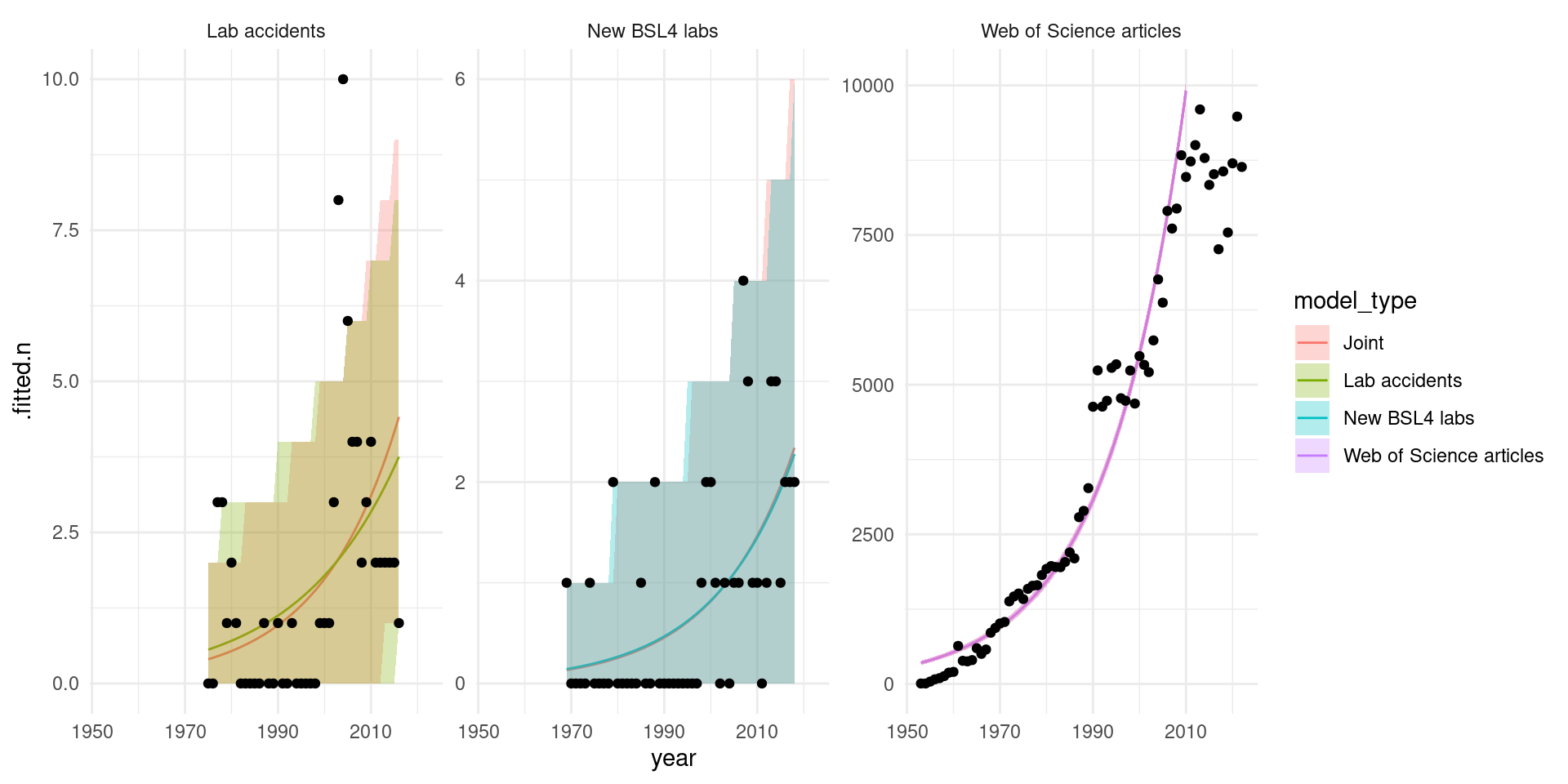
Poisson regression from fitting to each time series either individually or jointly (jointly assumes the same growth rate).
p = tbl_models |>
    filter(model_type == "Joint") |>
    unnest(fit_aug) |>
    mutate(
        .fitted.n = exp(.fitted),
        ymin = qpois(0.025, exp(.fitted)),
        ymax = qpois(0.975, exp(.fitted)),
    ) |>
    # mutate(across(c(ymin, ymax, n, .fitted.n), ~.x / max(n)), .by = type) |>
    ggplot(aes(year, .fitted.n)) +
    geom_line() +
    geom_ribbon(
        aes(year, ymin = ymin, ymax = ymax),
        alpha = 0.3,
    ) +
    geom_point(aes(year, n), data = all_counts) +
    facet_wrap(~type, scales = "free_y") +
    theme_minimal() +
    labs(
        x = "Year",
        y = "Number of events"
    )
    ggsave(
        here::here("docs/poisson-regression.png"),
        plot = p,
        width = 15,
        height = 10,
        units = "cm",
        dpi = 200
    )
tbl_models |>
unnest(fit_tidy) |>
filter(term == "year") |>
ggplot(aes(estimate, model_type, xmin = estimate - 1.96 * std.error, xmax = estimate + 1.96 * std.error)) +
geom_pointrange() +
theme_minimal() +
labs(
x = "Growth rate",
y = "Model"
)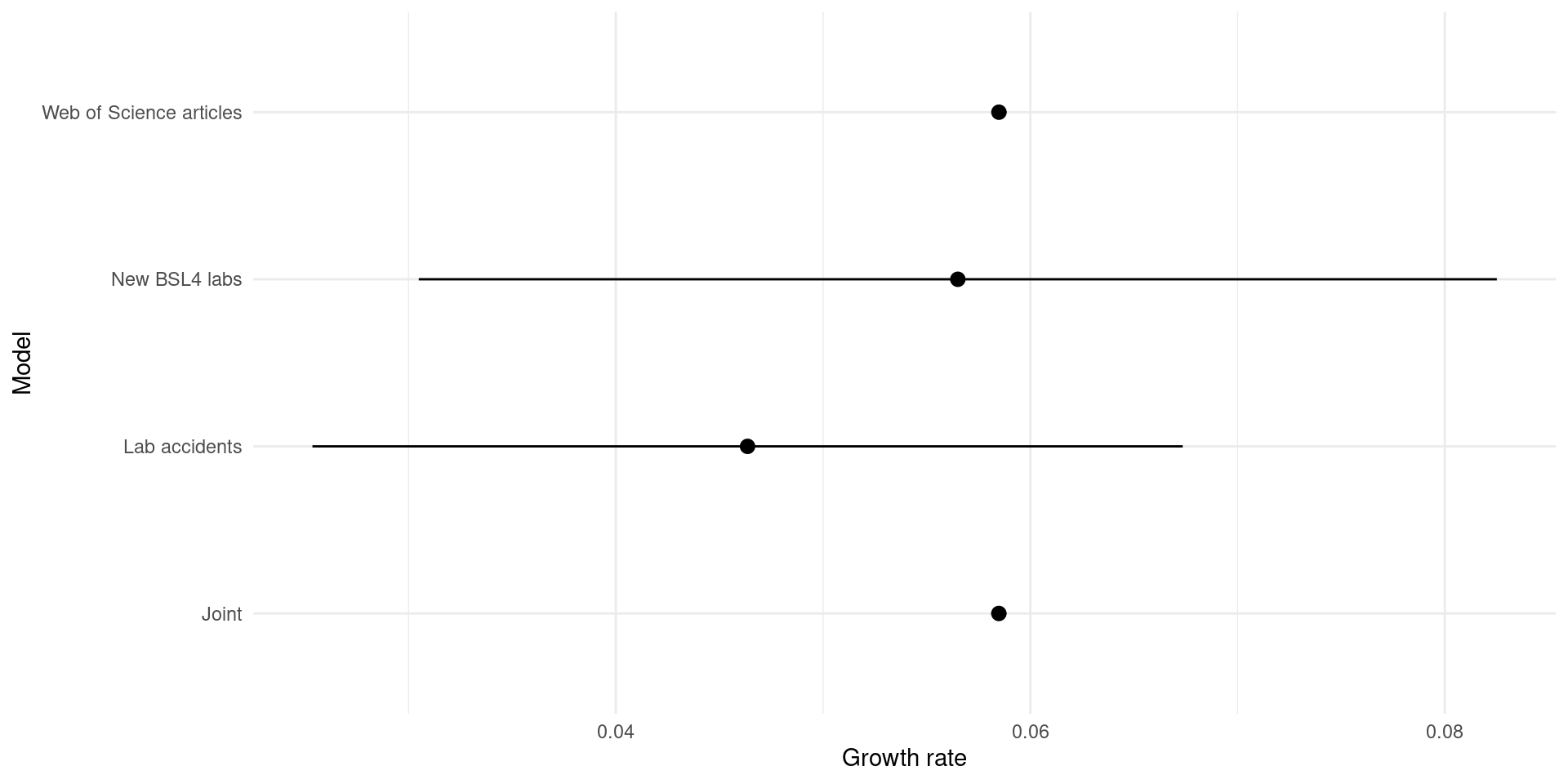
Growth rates from fitting to each time series either individually or jointly.
Forecast
One lab risk pandemic has occurred to date: the 1977 Russian flu pandemic. COVID-19’s origin is debated, and I present either scenario.
The forecast will be based on three quantities. These can be calculated from the historic record, and the growth rate of risky research units \(r\) estimated above.
- The number of risky research units conducted up until the time used for calculating the base rate, \(t_b\). We will normalize this to 1, meaning that we define the number of units as \(u(t) = r \exp(r(t-t_b))\). This gives the total risky research units conducted up until \(t_b\) as \(\int_{-\infty}^{t_b} u(t) dt = \exp(0) - \exp(-\infty) = 1\).
- The number of risky research units conducted in the period we are predicting, from \(t_0\) for \(d\) years. This is \(u_p = \int_{t_0}^{t_0+d} u(t) dt = \exp(r(t_0+d-t_b)) - \exp(r(t_0-t_b)) = \exp(r(t_0-t_b)) (\exp(rd) - 1)\).
- The number of lab-leak pandemics that have occurred in the period used for calculating the base rate.
The estimate for the expected number of lab-leak pandemics per risky research unit (using a Gamma(1/3, 1/3) prior) is Gamma(a+1/3, 1). The expected number of lab-leak pandemics over the period of interest is \(u_p(a + 1/3)\). The probability of there being at least one pandemic is \(1 - 1 / (1 + u_p)^(a + 1/3)\). See here for justification of the prior and the formulae giving these results.
This gives the following results, with r = 0.0584812 (a 2.5% increase per year).
r = final_growth_rate
leak_risks = tribble(
    ~Scenario, ~a, ~tb,
    "No pandemics", 0, 2023,
    "Pre-COVID", 1, 2019,
    "COVID zoonotic", 1, 2023,
    "COVID lab-leak", 2, 2023,
) |>
    mutate(
        t0 = 2024,
        d = 10,
    ) |>
    add_row(
        Scenario = "Risk between 1977 and now",
        a = 1,
        tb = 1977,
        t0 = 1978,
        d = 2024 - 1978,
    ) |>
    mutate(
        up = exp(r * (t0 - tb)) * (expm1(r * d)),
        E_lab_leaks = up * (a + 1/3),
        p_gte1_lab_leaks = 1 - 1 / (1 + up) ^ (a + 1/3),
    )
leak_risks
Full probability distributions
prob_dist = leak_risks |>
    cross_join(tibble(n = 0:59)) |>
    mutate(p = dnbinom(n, a + 1/3, 1 / (up + 1))) |>
    pivot_wider(
        names_from = Scenario,
        id_cols = n,
        values_from = p,
    )
prob_dist
Cumulative distribution
prob_dist |>
    mutate(across(-n, cumsum))
For comparison, Marani et al. (2021) suggests 2.5 zoonotic pandemics per decade, although this rate may have decreased since World War II.
Below I show how the rate is changing over time due to the change in risky research units.
p_gg = leak_risks |>
    cross_join(tibble(time = 2010:2050)) |>
    mutate(
        E_lab_leak_pandemics = r * exp(r * (time - tb)) * (a + 1/3),
    ) |>
    ggplot(aes(time, E_lab_leak_pandemics, color = Scenario)) +
    geom_line() +
    geom_hline(aes(colour = "E(zoonotic pandemics)", yintercept = 0.25)) +
    theme_minimal()
plotly::ggplotly(p_gg)
p = leak_risks |>
mutate(
n_prev = case_match(
Scenario,
"COVID zoonotic" ~ "1 previous lab leak",
"COVID lab-leak" ~ "2 previous lab leaks",
) |>
as.factor(),
) |>
filter(!is.na(n_prev)) |>
cross_join(tibble(time = 2010:2035)) |>
mutate(
E_lab_leak_pandemics = r * exp(r * (time - tb)) * (a + 1/3),
) |>
ggplot(aes(time, E_lab_leak_pandemics, color = n_prev)) +
geom_line() +
geom_hline(aes(colour = "Historic average", yintercept = 0.25)) +
theme_minimal() +
labs(
x = "Year",
y = "Expected number of pandemics",
colour = ""
) +
theme(legend.position = "bottom")
ggsave(
here::here("docs/forecast.png"),
plot = p,
width = 15,
height = 10,
units = "cm",
dpi = 200
)